computing

CECAM Macromolecular simulation software workshop

I’m co-organiser of this slightly-different  in October 2023 at the Forschungszentrum Jülich, Germany. Rather than following the traditional format of 3-4 day populated by talks with the odd poster session, this is an extended workshop made up of six mini-workshops. Since it is focussed on python-based tools for biomolecular simulations, of which there are an increasing number, the first mini-workshop will be a bootcamp that I will be lead instructor on (helped by David Dotson from ASU). I’m also leading the next mini-workshop on analysing biomolecular simulation data.

New Publication: Alchembed

In much of my research I’ve looked at how proteins embedded in cell membranes behave. An important part in any simulation of a membrane protein is, obviously, putting it into a model membrane, often a square patch of several hundred lipid molecules. This is surprisingly difficult: although a slew of methods have been published, none of them can embed several proteins simultaneously into a complex (non-flat) arrangement of lipids. For example, a virus, as shown in our recent paper.

Here we introduce a new method, dubbed Alchembed, that uses an alternative way, borrowed from free energy calculations, of “turning on�? the van der Waals interactions between the protein and the rest of the system. We show how it can be used to embed five different proteins into a model vesicle on a standard workstation. If you want to try it out, there is a on GitHub. This assumes you have is setup


You can get the paper for free from .

Is Software a Method?

Last month I went to the . As a   I was interested not only in my research area, but also in how my community viewed software. Were there talks and posters on how people had improved important pieces of community software? After all, there would be talks and posters on improving experimental methods. Turns out, not so much. Click to read the full post.


HackDay: Data on Acid

Every year the (SSI) run a brilliant meeting called the , usually in Oxford. This is an lasting two days. At first glance it doesn’t look like it would be relevant to my research, but I always learn something new, meet interesting people and start, well, collaborations. The latest edition was last week and was the fourth I’ve attended. (Disclaimer: for the last year-and-a-bit I’ve been which has been very useful – this is how I managed to train up to be a Software Carpentry Instructor. Alas my tenure has now ended).

For the last two years the workshop has been followed by a hackday which I’ve attended. Now I’m not a software developer, I’m a research scientist who uses million-line community-developed codes (like GROMACS and NAMD), but I do write code, often python, to analyse my simulations and also to automate my workflows. A hackday therefore, where many of the participants are research software engineers, pushes me clear out of my comfort zone. I remember last year trying to write python to access GitHub using its and thinking “I’ve never done anything like this before and I’ve no idea what to do.�?. This year was no different, except I’d pitched the idea so felt responsible for the success of the project.

The name of the project, , was suggested by Boris Adryan and the team comprised myself, , , and . The input was data produced by a proof of principle project I’ve run to test if I can predict whether individual mutations to S.aureus DHFR cause resistance to trimethoprim. The idea was to then turn it into abstract forms, either visual or sound, so you can get an intuitive feel for the data. Or it could just be aesthetic.

To cut a long story short, we did it, it is up and we came third in the competition! In the long term I’d like to develop it further and incorporate it into my volunteer crowd-sourced project, , that aims to predict whether bacterial mutations cause antibiotic resistance or not (when it is funded that is).

Installing GROMACS with MPI support on a Mac

GROMACS is an optimised molecular dynamics code, primarily used for simulating the behaviour of proteins. To compile GROMACS you need, well, some compilers. I install gcc using . Note that this requires you to . Then it is easy to install gcc version 4.9 by

sudo port install gcc49

(and yes, I know about , but I still find has more of the things I want than brew). So, once you’ve done a bit of preparation, on a Mac is easy. Once you’ve downloaded the source code tar ball.

tar xvf gromacs-5.0.2.tar.gz
cd gromacs-5.0.2
mkdir build
cmake .. -DGMX_BUILD_OWN_FFTW=ON -DCMAKE_INSTALL_PREFIX='/usr/local/gromacs/5.0.2/‘
make
sudo make install

Note that this will install it in /usr/local/gromacs/5.0.2 so you can keep multiple versions on the same machine and swap between them in a sane way by sourcing the GMRXC file, for example

source /usr/local/gromacs/4.6.7/bin/GMXRC

Adding MPI support on a Mac is trickier. This appears mainly to be because the gcc compilers from MacPorts (or clang from Xcode) don’t appear to support OpenMPI. You will know because when you run the cmake command you get a load of failures starting about ten lines down, such as

-- Performing Test OpenMP_FLAG_DETECTED - Failure

I managed to get a working version using the following approach; it is likely there are better (if you know, please leave a comment), but it has the virtue of working. First we need to install OpenMPI.

sudo port install openmpi

Now we need a compiler that supports OpenMPI. If you dig around in the MacPorts tree you can find some.

sudo port install openmpi-devel-gcc49

Finally, we can follow the steps above (I just mkdir build-mpi subfolder in the above source folder and then cd to it), but now we need a (slightly) complex cmake instruction

cmake .. -DGMX_BUILD_OWN_FFTW=ON
-DGMX_BUILD_MDRUN_ONLY=on
-DCMAKE_INSTALL_PREFIX=/usr/local/gromacs/5.0.2
-DGMX_MPI=ON -DCMAKE_C_COMPILER=mpicc-openmpi-devel-gcc49
-DCMAKE_CXX_COMPILER=mpicxx-openmpi-devel-gcc49
-DGMX_SIMD=SSE4.1

This is only going to build an MPI version of mdrun (which makes sense) and will install mdrun_mpi alongside the regular compiled binaries we did first. We have to tell cmake what all the new fancy compilers are called and, unfortunately, these don’t support AVX SIMD instructions so we have to fall back to SSE4.1. Experience suggests this doesn’t impact performance as much as you might think. Now you can run things like on your workstation!

A simple tutorial on analysing membrane protein simulations.

I’m teaching on how to analyse membrane protein simulations next week at the University of Bristol as part of a arranged by . As it is only 90 minutes long, it only covers two simple tasks but I show how you can do both with (a python module) or in Tcl in . Rather than write something and just distribute it to the people who are coming to the course, I’ve put the whole tutorial, including trajectory files and all the example code . Please feel free to clone it, make changes and send a pull request (or just send me any comments).

Getting an ext3 Drobo 5D to play nicely with Ubuntu 12.04

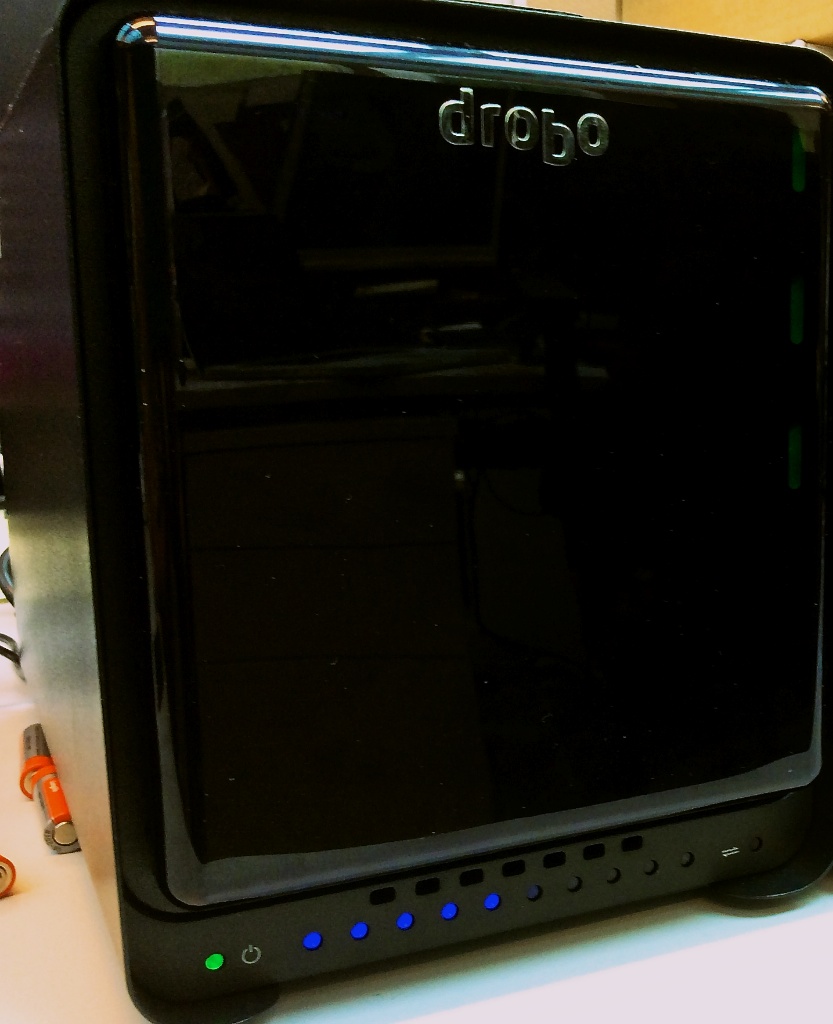
Our lab has recently bought two to give us some large storage. They work out of the box with Macs but getting them to play nicely with Linux, specifically Ubuntu 12.04, has been a bit more work so I thought I’d share the recipe that, for us at least, appears to work. Much of this has been cobbled together from the page and also from a very helpful earlier . One thing I could not get to work, unfortunately, is USB3. There appeared to be problems with USB3 and Linux when I was trying this out. Finally I should mention that the Drobo here was setup on a Mac, so was formatted HFS+ to begin with and, of course, follow these commands at your own risk. They worked for me, but they might not work for you..


First plug the Drobo into the power and connect with the USB lead to your Ubuntu machine. Don’t use any blue USB ports – these are USB3 and I couldn’t get them to work with the Drobo. After a while the Drobo should appear as a USB disk drive in a window. You can check what Ubuntu is doing by looking at this log

$ dmesg | tail

It will show something like

[250886.772714] usb 1-1.1: new high-speed USB device number 10 using ehci_hcd
[250887.331458] scsi19 : usb-storage 1-1.1:1.0
[250888.328628] scsi 19:0:0:0: Direct-Access Drobo 5D 5.00 PQ: 0 ANSI: 0
[250888.329605] sd 19:0:0:0: Attached scsi generic sg3 type 0
[250888.330168] sd 19:0:0:0: [sdb] Very big device. Trying to use READ CAPACITY(16).

First we need to intall the latest version of the linux Drobo tools, so we will probably need git and let’s get QT as well so we can check the GUI.

$ sudo apt-get install git
$ sudo apt-get install python-qt4

Now cd to somewhere where you put packages etc and run

$ git clone git://drobo-utils.git.sourceforge.net/gitroot/drobo-utils/drobo-utils

This will download all the files and binaries you need

$ cd drobo-utils/

Just check it is all up to date

$ git pull

Check it is all working by seeing if this works (warning: this can take about a minute)

$ sudo ./drobom status

In theory, we can bring up the GUI as below, but on my machine I just got python errors about KeyError: 'UseStaticIPAddress'. Check it if you want.

$ sudo ./drobom view

Next we need to know which device the Drobo is currently plugged into. This will probably change everytime you plug the Drobo in.

$ ls -lrt /dev/disk/by-uuid/

There should be a long alphanumeric list that I will call foo that is pointing to something like /dev/sdb. The foo should match the foo when I type

$ ls /media/

If so, then we know that the Drobo is connected to /dev/sdb. Next we need to set the Logical Unit Size (LUNS). This is the largest volume the Drobo will appear as, and if we run a df it will show this as the physical size of the Drobo even if there are not enough disks inside to make it this size. Since the Drobo 5D has five slots and we are using 4TB disks at present, then if we run with single disk redundancy the maximum size is 16 TB. You could make this smaller but then you would have multiple “drobo partitions�? mounted all pointing to the same machine. The disadvantage with a large LUNS is it means the startup time is long, as is any disk checking time. The units in the line below are TB! Caution these commands can take a while to run and I’ve not pasted in the usual “are you sure?�? prompts.

$ sudo ./drobom set lunsize 16 PleaseEraseMyData

Now we need to setup a partition for the disk using parted which should be already installed. This has its own command line. Although we are setting up an ext3 disk, it seems ext3 is just ext2 with journalling, so we ask parted for an ext2 disk.

$ sudo parted /dev/sdb
GNU Parted 1.8.9
Using /dev/sdd
Welcome to GNU Parted! Type 'help' to view a list of commands.
(parted) mklabel
New disk label type? gpt
(parted) mkpart ext2 0 100%
(parted) quit
Information: You may need to update /etc/fstab.

Now we need to format the disk. Again remember to use the right device. Also note it is sdb1 since we are formatting the first and only partition, not the disk itself. Also note again we are formatting as ext2 but with the -j flag for journalling, hence ext3. Again, this will ask whether you are sure etc and could take a few hours.

$ sudo mke2fs -j -i 262144 -L Drobo -m 0 -O sparse_super,^resize_inode /dev/sdb1

Nearly there. If you remount the Drobo it should appear in /Media/Drobo (or whatever name you gave it above) Now we need to make sure you have permissions to write to the disk. For this we need to know your user and group numeric ids.

$ id
uid=9009(fowler) gid=100 groups=100

So my user id is 9009 and my group id is 100. Hence

$ sudo chown -R 9009:100 /media/Drobo/

If we want to mount the Drobo somewhere else, we need to edit /etc/fstab. First we need to know the UUID of the disk (this was the foo).

$ ls -lrt /dev/disk/by-uuid/

Copy the foo into the clipboard and open

$ sudo emacs /etc/fstab

Add a line at the end that looks like

# mount the ext3 Drobo
UUID=b278aff6-db1a-436b-995b-8808c2c82f9e /drobo1 ext3 defaults 0 2

make sure the mount point exists!

$ sudo mkdir /drobo1

Now remount the disk, either by rebooting or by issuing

$ sudo mount -a

and voila, you should find the disk by

$ ls /drobo1/

Check you can make a file

$ touch /drobo1/hello-world.txt

Check it appears in your list of disks using df etc. I’ve checked you can be a bit rough with it e.g. just pulling out the USB cable and then reconnecting to a different port. Seemed ok but I did need to remount it using

$ sudo mount -a

and then I could add and edit files as normal and there was no complaining in dmesg about write-only filesystems or anything like before with HFS+.

GROMACS 4.6: Running on GPUs

I mentioned before that I would write something on running on GPUs. Let’s imagine we want to simulate a solvated lipid bilayer containing 6,000 lipids for 5 µs. The total number of is around 137,000 and the box dimensions are roughly 42x42x11 nm. Although this is smaller than the benchmark we looked at last time, it is still a challenge to run on a workstation. To see this let’s consider running it on my MacPro using GROMACS 4.6.1. The machine is an and has 2 Intel Xeons, each with 4 cores. Using 8 MPI processes gets me 132 ns/day, so I would have to wait 38 days for 5 µs. Too slow!


You have to be careful installing non-Apple supported NVidia GPUs into MacPros, not least because you are limited to 2x6pin power connectors. Taking all this into account, the best I can do without doing something drastic to the power supply is to install an . Since I only have one GPU, I can only run one MPI process, but this can spawn multiple OpenMP threads. For this particular system, I get the best performance with 4 threads (134 ns/day) which is the same performance I get using all 8 cores without the GPU. So when I am using just a single core, adding in the GPU increases the performance by a factor of 3.3x. But as I add additional cores, the increase afforded by the single GPU drops until the performance is about the same at 8 cores.

Now let’s try something bigger. Our lab has a small Intel (Sandy Bridge) computing cluster. Each node has 12 cores, and there are 8 nodes, yielding a maximum of 96 cores. Running on the whole cluster would reduce the time down to 6 days, which is a lot better but not very fair on everyone else in the lab. We could try and get access to Tier-1 or Tier-0 supercomputers but, for this system, that is overkill. Instead let’s look at a Tier-2 machine that uses GPUs to accelerate the calculations.


fig-blog-gpu-5

The University of Oxford, through , has access to the machines owned by the Centre for Innovation. One of these, , is a GPU-based cluster. We shall look at one of the partitions; this has 60 nodes, each with two 6-core Intel processors and 3 NVIDIA M2090 Tesla GPUs. For comparison, let’s run without the GPUs. The data shown are for simulations with only 1 OpenMP thread per MPI process. So now let’s run using the GPUs (which is the point of this cluster!). Again just using asingle OpenMP thread per MPI process/GPU (shown on graph) we again find a performance increase of 3-4x. Since there are 3 GPUs per node, and each node has 12 cores, we could run 3 MPI processes (each attached to a GPU) on each node and each process could spawn 1, 2, 3 or 4 OpenMP threads. This uses more cores,  but since they probably would be sitting idle, this is a more efficient use of the compute resource. Trying 2 or 3 OpenMP threads per MPI process/GPU lets us reach a maximum performance of 1.77 µs per day, so we would get our 5 µs in less than 3 days. Comparing back to our cluster, we can get the same performance of our 96-core local cluster using a total of 9 GPUs and 18 cores on EMERALD.

Finally, let’s compare EMERALD to the Tier-1 PRACE supercomputer CURIE. CURIE was the . For this comparison we will need to use a bigger benchmark, so let’s us . It has 9x the number of lipids, but because I had to add extra water ends up being about 15x bigger at 2.1 million particles. Using 24 GPUs and 72 cores, EMERALD manages 130 ns/day. To get the same performance on CURIE requires 150 cores and ultimately CURIE tops out at 1,500 ns/day on 4,196 cores. Still, EMERALD is respectable and shows how it can serve as a useful bridge to Tier-1 and Tier-0 supercomputers. Interestingly, CURIE also has a “hybrid�? partition that contains 144 nodes, each with 2 Intel Westmere processors and 2 NVIDIA M2090 Tesler GPUs. I was able to run on up to 128 GPUs with 4 OpenMP threads per MPI/GPU, making a total of 512 cores. This demonstrates that GROMACS can run on large numbers of GPU/CPUs and that such hybrid architectures are viable as supercomputers (for GROMACS at least).

GROMACS 4.6: Scaling of a very large coarse-grained system

So if I have a particular system I want to simulate, how many processing cores can I harness to run a single version 4.6 job? If I only use a few then the simulation will take a long time to finish, if I use too many the cores will end up waiting for communications from other cores and so the simulation will be inefficient (and also take a long time to finish). In between is a regime where the code, in this case GROMACS, scales well. Ideally, of course, you’d like linear scaling i.e. if I run on 100 cores in parallel it is 100x faster than if I ran on just one.

The rule of thumb for GROMACS 4.6 is that it scales well until there are only ~130 atoms/core. In other words, the more atoms or beads in your system, the larger the number of computing cores you can run on before the scaling performance starts to degrade.

As you might imagine there is a hierarchy of computers we can run our simulations on; this starts at humble workstations, passes through departmental, university and regional computing clusters before ending up at national (Tier 1) and international (Tier 0) high performance computers (HPC).

In our lab we applied for, and , a set of European Tier 0 supercomputers through PRACE. These are currently amongst the . We tested five supercomputers in all: (Paris, France; green lines), (Barcelona, Spain; black line), (Bologna, Italy; lilac), (Munich, Germany; blue) and (Stuttgart, Germany; red ). Each has a different architecture and inevitably some are slightly newer than others. CURIE has three different partitions, called thin, fat and hybrid. The thin nodes constitute the bulk of the system; the fat nodes have more cores per node whilst the hybrid nodes combine conventional CPUs with GPUs.

We tested a coarse-grained 54,000 lipid bilayer (2.1 million beads) on all seven different architectures and the performance is shown in the graph – note that the axes are logarithmic. Some machines did better than others; FERMI, which is an , appears not to be well-suited to our benchmark system, but then one doesn’t expect fast per-core performance on a BlueGene as that is not how they are designed. Of the others, MareNostrum was fastest for small numbers of cores, but its performance began to suffer if more than 256 cores were used. SuperMUC and the Curie thin nodes were the fastest conventional supercomputers, with the Curie thin nodes performing better at large core counts. Interestingly, the Curie hybrid GPU nodes were very fast, especially bearing in mind the CPUs on these nodes are older and slower than those in the thin nodes. One innovation introduced into GROMACS 4.6 that I haven’t discussed previously is one can now run either using purely MPI processes or a . We were somewhat surprised to find, that, in nearly all cases, the pure MPI approach remained slightly faster than the new hybrid parallelisation.

Of course, you may see very different performance using your system with GROMACS 4.6. You just have to try and see what you get! In the next post I will show some detailed results on using GROMACS on GPUs.